


Abstract
Despite the growing popularity of propensity score (PS) methods in epidemiology, relatively little has been written in the epidemiologic literature about the problem of variable selection for PS models. The authors present the results of two simulation studies designed to help epidemiologists gain insight into the variable selection problem in a PS analysis. The simulation studies illustrate how the choice of variables that are included in a PS model can affect the bias, variance, and mean squared error of an estimated exposure effect. The results suggest that variables that are unrelated to the exposure but related to the outcome should always be included in a PS model. The inclusion of these variables will decrease the variance of an estimated exposure effect without increasing bias. In contrast, including variables that are related to the exposure but not to the outcome will increase the variance of the estimated exposure effect without decreasing bias. In very small studies, the inclusion of variables that are strongly related to the exposure but only weakly related to the outcome can be detrimental to an estimate in a mean squared error sense. The addition of these variables removes only a small amount of bias but can increase the variance of the estimated exposure effect. These simulation studies and other analytical results suggest that standard model-building tools designed to create good predictive models of the exposure will not always lead to optimal PS models, particularly in small studies.
Propensity score (PS) methods, as formalized by Rosenbaum and Rubin (1), are becoming standard techniques for controlling confounding in nonexperimental studies in medicine and epidemiology. Unlike conventional statistical approaches that depend on a model of the outcome under study, PS methods rely on a model of the exposure or treatment (termed “the PS model”). A central issue facing researchers using PS methods is how to select the variables to be included in the PS model. Ideally, specification of the model will be guided by knowledge of the subject matter—for example, a detailed understanding of how a particular treatment is assigned to patients. Frequently, however, the researcher does not have the benefit of such knowledge and instead is confronted with a large collection of pretreatment covariates and many derived functions of these covariates (e.g., interactions) and must decide which of these terms to enter into a regression model of the exposure. The bias and variance of the estimated exposure effect can depend strongly on which of these candidate variables are included in the PS model.
Despite the growing popularity of PS methods, relatively little has been written about the variable selection problem for PS models. In the context of multivariate normal confounders, Rubin and Thomas (2) derived approximations for the reduction in the bias and variance of an estimated exposure effect from PS-matched analysis. They suggest including in a PS model all variables thought to be related to the outcome, whether or not they are related to exposure (2). In a later paper, Rubin (3) suggests that including variables that are strongly related to exposure but unrelated to the outcome can decrease the efficiency of an estimated exposure effect; but he argues that if such a variable had even a weak effect on the outcome, the bias resulting from its exclusion would dominate any loss of efficiency for a reasonable-sized study. Some of these guidelines are repeated by Perkins et al. (4). Robins et al. (5) derived analytical results showing that the asymptotic variance of an estimator based on an exposure model is not increased and is often decreased as the number of parameters in the exposure model is increased. These results suggest that the size of a PS model should increase with the study size. Hirano and Imbens (6) proposed a variable selection strategy for use with a multivariable outcome model employing PS weighting.
In practice, variables are often selected in data-driven ways—for example, by using stepwise variable selection algorithms to develop good predictive models of the exposure (7). Furthermore, in many PS analyses, investigators report the c statistic (the area under the receiver operating characteristic curve) for the final PS model as a means of assessing the model's adequacy (7, 8). Implicit in this practice is the assumption that PS models that are better predictors or discriminators of the exposure status result in superior estimators of exposure effect. According to this criterion, any variable that increases the c statistic or predictive ability of the PS model should be selected for inclusion in the model. Despite the widespread use of such variable selection strategies, there has been little discussion of their appropriateness. In a recent editorial, Rubin (9) expressed doubt over the usefulness of such diagnostics in a PS analysis.
We conducted the present work to illuminate this issue and to help researchers gain some practical insight into the variable selection problem in a PS analysis. We present the results of two Monte Carlo simulation experiments designed to evaluate how different specifications of a PS model affect the bias, variance, and resulting mean squared error (MSE) of an estimated exposure effect under a variety of assumptions about the data-generating process.
MATERIALS AND METHODS
Brief overview of PS methods
In many nonexperimental cohort studies in medicine and epidemiology, the relation between an exposure A and an outcome Y may be confounded by a set of measured baseline variables X = (X1, X2, …, Xp). As potential confounders, the elements of X can be both predictors of the exposure and independent risk factors for the outcome. As an illustration, consider an observational cohort study in which the exposure of interest is the use of a particular cholesterol-lowering drug at the start of the study and the outcome is having a myocardial infarction during the follow-up period. The potential confounders that are measured at the start of the study include age, gender, lipid levels, comorbid conditions, previous drug exposures, and diet and exercise habits. For such studies, statistical methods based on the PS can be used to estimate exposure effects.
The PS is the conditional probability that a subject receives a treatment or exposure under study given all measured confounders, that is, Pr[A = 1|X]. The PS has been termed a balancing score, meaning that among subjects with the same propensity to be exposed, treatment is conditionally independent of the covariates (1). This balancing property suggests that estimates of the exposure effect that are not confounded by any of the measured covariates can be obtained by estimating the effect of exposure within groups of people with the same PS. Within such a group, any difference in outcome between the exposed and unexposed subjects is not attributable to the measured confounders. If treatment assignment is strongly ignorable and other specific assumptions hold, estimates derived from a PS analysis can be interpreted causally (1).
In most nonexperimental research, the true PS will not be known and therefore will need to be estimated, typically according to an assumed model. The bias and variance of the estimated exposure effect can depend strongly on how the model of Pr[A = 1|X] is specified. The model specification problem includes selecting variables from X to be included in the model and deciding how the variables are to be transformed, categorized, and interacted with one another.
Given an estimated PS, exposure effects are usually estimated by either 1) matching exposed subjects with unexposed subjects on the PS to create two comparable groups, 2) including the PS and the exposure in a multivariable model of the outcome under study, or 3) conducting an analysis stratified across categories of the PS. It is also possible to use the PS to generate inverse-probability-of-exposure weights that are then used in a weighted regression (10). The weighting approach generalizes naturally to longitudinal data with time-varying treatments and confounders. More detailed discussions of PS methods can be found elsewhere (1, 11, 12).
Monte Carlo simulation study
To explore the variable selection problem in PS models, we performed two Monte Carlo simulation experiments. The first examined how the inclusion of three different types of covariates in a PS model affected the estimated exposure effect (see figure 1): 1) a variable related to both outcome and exposure—a true confounder (X1); 2) a variable related to the outcome but not the exposure (X2); and 3) a variable related to the exposure but not the outcome (X3). In the second experiment, we considered how the addition of a single confounder to a PS model changes the bias and variance of an estimated exposure effect under varying assumptions about the strength of the confounder-outcome and confounder-exposure relations.
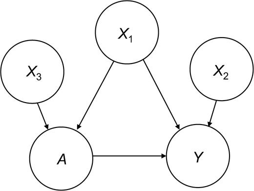
Causal diagram for simulation experiment 1.
Both simulation experiments employed the same basic data-generating process. The simulated data consisted of realizations of a dichotomous exposure, an outcome with a Poisson distribution, and continuous confounders. The data were generated in the following order according to the specified probability models:
The covariates X1, X2, and X3 are independent standard normal random variables with mean 0 and unit variance.
- The conditional distribution of the dichotomous exposure A given X1, X2, and X3 follows a Bernoulli distribution with a conditional mean given by the functionwhere Φ is the standard normal cumulative distribution function.\[\mathrm{Pr}{[}A{=}1{\vert}X_{1},{\,}X_{2},{\,}X_{3}{]}{=}{\Phi}(\mathrm{{\beta}}_{0}{+}\mathrm{{\beta}}_{1}X_{1}{+}\mathrm{{\beta}}_{2}X_{2}{+}\mathrm{{\beta}}_{3}X_{3}),\]
- The conditional distribution of Y given X and A follows a Poisson distribution with two possible specifications of the mean. The first specification (used in the first simulation experiment) is given byThis specification creates a nonlinear (S-shaped) relation between the confounder X1 and the log of the expected value of the outcome. The second specification (used in the second simulation experiment) is given by\begin{eqnarray*}&&\mathbf{\mathrm{E}}{[}Y{\vert}A,{\,}X_{1},{\,}X_{2},{\,}X_{3}{]}{=}\mathrm{exp}{\{}\mathrm{{\alpha}}_{0}{+}\mathrm{{\alpha}}_{1}((1{+}\mathrm{exp}({-}3{\times}X_{1}))^{{-}1}\\&&{-}0.5){+}\mathrm{{\alpha}}_{2}X_{2}{+}\mathrm{{\alpha}}_{3}X_{3}{+}\mathrm{{\alpha}}_{4}A{\}}.\end{eqnarray*}This model specifies a standard log-linear relation between the covariates and the outcome.\begin{eqnarray*}&&\mathbf{\mathrm{E}}{[}Y{\vert}A,{\,}X_{1},{\,}X_{2},{\,}X_{3}{]}{=}\mathrm{exp}{\{}\mathrm{{\alpha}}_{0}{+}\mathrm{{\alpha}}_{1}X_{1}{+}\mathrm{{\alpha}}_{2}X_{2}\\&&{+}\mathrm{{\alpha}}_{3}X_{3}{+}\mathrm{{\alpha}}_{4}A{\}}.\end{eqnarray*}
Within both simulation experiments, the effect of exposure is held constant (α4 = 0.5). The simulations differ in how the covariates are related to the exposure and outcome.
Evaluation of PS model performance
Simulation experiment 1
For this experiment, exposure was confounded through X1, X3 predicted treatment but was unrelated to the outcome, and X2 predicted the outcome but was unrelated to treatment (α0 = 0.5, α1 = 4, α2 = 1, α3 = 0, β0 = 0, β1 = 0.5, β2 = 0, β3 = 0.75). This scenario is depicted graphically in figure 1.
We simulated 1,000 data sets for both n = 500 and n = 2,500. For each simulated data set, we estimated seven different PS's corresponding to all possible combinations of X1, X2, and X3 in a probit regression model. These models are given byFor each PS model, we report the estimated bias, variance, and MSE of the corresponding estimator. We also report these statistics for the simple estimator corresponding to the crude log relative rate. To assess the predictive ability of each PS model, we additionally report the average c statistic for the model across simulations. The c statistic is computed by forming all discordant pairs of observations (exposed and unexposed combinations) and computing the proportion of these pairs in which the exposed subject had a higher estimated PS than the unexposed subject (15).
PS model 1: Pr[A = 1|X] = Φ(β0 + β1X1).
PS model 2: Pr[A = 1|X] = Φ(β0 + β1X2).
PS model 3: Pr[A = 1|X] = Φ(β0 + β1X3).
PS model 4: Pr[A = 1|X] = Φ(β0 + β1X1 + β2X2).
PS model 5: Pr[A = 1|X] = Φ(β0 + β1X1 + β2X3).
PS model 6: Pr[A = 1|X] = Φ(β0 + β1X2 + β2X3).
PS model 7: Pr[A = 1|X] = Φ(β0 + β1X1 + β2X2 + β3X3).
We conducted a variety of sensitivity analyses with n = 500. These analyses were carried out by holding all parameters at their default values while a single parameter was altered. The following sensitivity analyses were performed: The standard deviation of each covariate was both increased by 50 percent and decreased by 50 percent; the treatment effect was decreased to α4 = 0.25 and increased to α4 = 1; and the baseline prevalence of the exposure was decreased from approximately 50 percent to approximately 20 percent (β0 = −1).
Simulation experiment 2
In the second simulation experiment, we examined how the inclusion of a single true confounder in a PS model affected the bias and variance of an estimated exposure effect under varying assumptions about the strength of association between the single confounder and both the outcome and the exposure. For each simulated data set, two estimators were considered: The first was derived from the crude log relative rate, and the second was derived from a PS-adjusted estimate of the effect of A on Y in which the PS model contained only the confounder X1. In this simulation experiment, the adjustment for the PS used the spline approach. We denote the crude estimator of the log relative rate with
The parameter α1, the strength of association between X1 and Y, took values in the set {0, 0.01, …, 0.20}, corresponding to relative rates ranging from 1.00 to 1.28. The parameter β1, the strength of association between X1 and A, took values in the set {0.00, 0.05, …, 1.25}. For all possible combinations of these values of α1 and β1, we simulated 1,000 data sets of n = 500 and n = 2,500. In this simulation, the covariates X2 and X3 are not used. For each set of 1,000 data sets, we computed the estimated bias, variance, and MSE of each of the two estimators.
Computation
All simulations were performed in R, version 1.9.1 (16, 17), running on a Windows XP platform, using software created by one of the authors (M. A. B.).
RESULTS
Simulation experiment 1
For the simulations controlling for the PS through a spline, we report the estimated bias, variance, and MSE of all estimators in table 1. We also report the average c statistic for each candidate PS model. The sole confounder was the covariate X1; therefore, any estimator that did not contain X1 in the PS model was biased. For both study sizes, the unbiased estimator with the smallest variance was the one that contained the confounder X1 and the covariate related to the outcome only, X2. This estimator had approximately 30 percent (n = 500) and 25 percent (n = 2,500) less variance than the estimator containing just the confounder X1. Adding X3, the covariate related only to exposure, increased the variance of the estimated effect for both study sizes. The estimator with all covariates in the PS model had a variance that was approximately 40 percent greater (for both study sizes) than the estimator with just the covariates X1 and X2. The c statistic of the PS model with X1 and X2 was smaller (0.67) than the c statistic of the less efficient PS model with all covariates (≈0.8). For both study sizes, the PS models with the highest average c statistic contained all variables related to the exposure.
Simulation experiment 1, with results based on an analysis in which the propensity score is entered into an outcome model as a parametric spline term*
Variable(s) in propensity score model | |||||||||||||||
|---|---|---|---|---|---|---|---|---|---|---|---|---|---|---|---|
| X1 | X2 | X3 | X1, X2 | X1, X3 | X2, X3 | X1, X2, X3 | None | ||||||||
| n = 500 | |||||||||||||||
| Bias × 101 | −0.03 | 5.97 | 7.34 | −0.03 | −0.07 | 7.36 | −0.06 | 5.94 | |||||||
| Var × 101 | 0.32 | 0.22 | 0.46 | 0.22 | 0.44 | 0.36 | 0.31 | 0.39 | |||||||
| MSE × 101 | 0.32 | 3.79 | 5.85 | 0.22 | 0.44 | 5.77 | 0.31 | 3.92 | |||||||
| Average c statistic | 0.67 | 0.52 | 0.76 | 0.67 | 0.82 | 0.76 | 0.82 | ||||||||
| n = 2,500 | |||||||||||||||
| Bias × 101 | 0.00 | 5.93 | 7.33 | −0.01 | −0.04 | 7.33 | −0.03 | 5.95 | |||||||
| Var × 102 | 0.66 | 0.53 | 0.96 | 0.49 | 0.89 | 0.79 | 0.69 | 0.80 | |||||||
| MSE × 102 | 0.66 | 35.65 | 54.72 | 0.49 | 0.89 | 54.56 | 0.70 | 36.16 | |||||||
| Average c statistic | 0.67 | 0.51 | 0.76 | 0.67 | 0.81 | 0.76 | 0.81 | ||||||||
The table shows the estimated bias, variance (Var), and mean squared error (MSE) of all possible estimators and the average c statistic for the corresponding propensity score model.
Table 2 shows the results obtained when this simulation experiment was repeated using subclassification instead of spline adjustment. The results were qualitatively similar, but there were some notable differences. The effect of adding X3 was more detrimental in a relative MSE sense. In addition, all unbiased estimators were considerably less variable than the corresponding estimators based on spline adjustment. Finally, all estimators admit some bias due to residual confounding within strata of the PS.
Simulation experiment 1, with results based on an analysis using subclassification in which strata are defined by quintiles of the estimated propensity score*
Variable(s) in propensity score model | |||||||||||||||
|---|---|---|---|---|---|---|---|---|---|---|---|---|---|---|---|
| X1 | X2 | X3 | X1, X2 | X1, X3 | X2, X3 | X1, X2, X3 | None | ||||||||
| n = 500 | |||||||||||||||
| Bias × 101 | 0.29 | 6.07 | 7.96 | 0.24 | 0.24 | 7.93 | 0.24 | 5.94 | |||||||
| Var × 101 | 0.22 | 0.14 | 0.62 | 0.16 | 0.71 | 0.43 | 0.69 | 0.39 | |||||||
| MSE × 101 | 0.23 | 3.82 | 6.95 | 0.17 | 0.71 | 6.71 | 0.70 | 3.92 | |||||||
| n = 2,500 | |||||||||||||||
| Bias × 101 | 0.28 | 5.96 | 7.61 | 0.29 | 0.55 | 7.60 | 0.56 | 5.95 | |||||||
| Var × 102 | 0.43 | 0.31 | 1.02 | 0.27 | 1.12 | 0.87 | 0.96 | 0.80 | |||||||
| MSE × 102 | 0.51 | 35.82 | 58.90 | 0.35 | 1.43 | 58.63 | 1.27 | 36.16 | |||||||
The table shows the estimated bias, variance (Var), and mean squared error (MSE) of all possible estimators.
The results of the sensitivity analysis are presented in table 3. In all of the sensitivity analyses, the same essential pattern prevailed: The inclusion of the variable related only to exposure increased the variance of the estimator without altering bias; inclusion of the variable related only to the outcome decreased variance without affecting bias; and failure to include the confounder yielded a biased estimator. However, the perturbation of simulation parameters changed absolute and, in some cases, relative numbers.
Sensitivity analysis of simulation study 1*
Parameter change | Variable(s) in propensity score model | ||||||||||||||
|---|---|---|---|---|---|---|---|---|---|---|---|---|---|---|---|
| X1 | X2 | X3 | X1, X2 | X1, X3 | X2, X3 | X1, X2, X3 | None | ||||||||
| Original | |||||||||||||||
| Bias × 101 | −0.03 | 5.97 | 7.34 | −0.03 | −0.07 | 7.36 | −0.06 | 5.94 | |||||||
| Var × 101 | 0.32 | 0.22 | 0.46 | 0.22 | 0.44 | 0.36 | 0.31 | 0.39 | |||||||
| MSE × 101 | 0.32 | 3.79 | 5.85 | 0.22 | 0.44 | 5.77 | 0.31 | 3.92 | |||||||
| Decrease in the variance of X1 | |||||||||||||||
| Bias × 101 | 0.13 | 2.94 | 3.81 | 0.12 | 0.13 | 3.80 | 0.12 | 2.99 | |||||||
| Var × 101 | 0.27 | 0.21 | 0.47 | 0.19 | 0.38 | 0.38 | 0.28 | 0.35 | |||||||
| MSE × 101 | 0.27 | 1.07 | 1.92 | 0.19 | 0.38 | 1.82 | 0.28 | 1.24 | |||||||
| Increase in the variance of X1 | |||||||||||||||
| Bias × 101 | 0.06 | 8.46 | 10.1 | 0.02 | 0.07 | 10.04 | 0.02 | 8.49 | |||||||
| Var × 101 | 0.38 | 0.28 | 0.50 | 0.27 | 0.51 | 0.41 | 0.38 | 0.44 | |||||||
| MSE × 101 | 0.38 | 7.44 | 10.71 | 0.27 | 0.51 | 10.50 | 0.38 | 7.64 | |||||||
| Decrease in the variance of X2 | |||||||||||||||
| Bias × 101 | 0.02 | 5.96 | 7.38 | 0.02 | 0.00 | 7.38 | 0.01 | 5.97 | |||||||
| Var × 101 | 0.07 | 0.13 | 0.19 | 0.05 | 0.12 | 0.17 | 0.10 | 0.16 | |||||||
| MSE × 101 | 0.07 | 3.69 | 5.64 | 0.05 | 0.12 | 5.62 | 0.10 | 3.72 | |||||||
| Increase in the variance of X2 | |||||||||||||||
| Bias × 101 | 0.23 | 6.16 | 7.59 | 0.19 | 0.24 | 7.53 | 0.18 | 6.16 | |||||||
| Var × 101 | 1.20 | 0.60 | 1.57 | 1.00 | 1.62 | 1.32 | 1.32 | 1.25 | |||||||
| MSE × 101 | 1.21 | 4.39 | 7.33 | 1.00 | 1.62 | 7.00 | 1.32 | 5.04 | |||||||
| Decrease in the variance of X3 | |||||||||||||||
| Bias × 101 | 0.08 | 6.89 | 7.35 | 0.03 | 0.04 | 7.30 | 0.02 | 6.94 | |||||||
| Var × 101 | 0.34 | 0.25 | 0.46 | 0.23 | 0.39 | 0.36 | 0.28 | 0.42 | |||||||
| MSE × 101 | 0.35 | 5.00 | 5.86 | 0.23 | 0.39 | 5.70 | 0.28 | 5.24 | |||||||
| Increase in the variance of X3 | |||||||||||||||
| Bias × 101 | 0.10 | 5.07 | 7.53 | 0.07 | 0.05 | 7.49 | 0.01 | 5.1 | |||||||
| Var × 101 | 0.29 | 0.23 | 0.55 | 0.21 | 0.49 | 0.46 | 0.39 | 0.38 | |||||||
| MSE × 101 | 0.29 | 2.80 | 6.21 | 0.22 | 0.49 | 6.07 | 0.39 | 2.98 | |||||||
| Decrease in α4, decrease in the treatment effect | |||||||||||||||
| Bias × 101 | 0.08 | 5.98 | 7.46 | 0.03 | 0.11 | 7.41 | 0.04 | 6.02 | |||||||
| Var × 101 | 0.32 | 0.24 | 0.47 | 0.22 | 0.43 | 0.37 | 0.31 | 0.39 | |||||||
| MSE × 101 | 0.32 | 3.82 | 6.03 | 0.22 | 0.43 | 5.86 | 0.31 | 4.01 | |||||||
| Increase in α4, increase in the treatment effect | |||||||||||||||
| Bias × 101 | −0.12 | 5.68 | 6.92 | −0.08 | −0.16 | 6.99 | −0.10 | 5.62 | |||||||
| Var × 101 | 0.34 | 0.21 | 0.52 | 0.23 | 0.49 | 0.39 | 0.33 | 0.38 | |||||||
| MSE × 101 | 0.34 | 3.43 | 5.32 | 0.23 | 0.49 | 5.27 | 0.34 | 3.54 | |||||||
| Decrease in β0, decrease in exposure prevalence | |||||||||||||||
| Bias × 101 | 0.03 | 6.02 | 7.34 | 0.00 | 0.01 | 7.35 | 0.00 | 5.99 | |||||||
| Var × 101 | 0.32 | 0.27 | 0.51 | 0.23 | 0.46 | 0.41 | 0.34 | 0.43 | |||||||
| MSE × 101 | 0.32 | 3.90 | 5.89 | 0.23 | 0.46 | 5.81 | 0.34 | 4.01 | |||||||
We consider nine different perturbations of the simulation parameters. Results are from 1,000 simulations of data (n = 500), using a parametric spline to adjust for the estimated propensity score. For each simulation, we report the estimated bias, variance (Var), and mean squared error (MSE) of the estimators corresponding to all possible specifications of the propensity score model.
Simulation experiment 2
In figure 2, we plot the estimated variance of the PS-adjusted estimator
![Variance of the unadjusted estimator \batchmode \documentclass[fleqn,10pt,legalpaper]{article} \usepackage{amssymb} \usepackage{amsfonts} \usepackage{amsmath} \pagestyle{empty} \begin{document} \(\mathrm{{\hat{{\gamma}}}}_{0}\) \end{document} and the propensity score-adjusted estimator \batchmode \documentclass[fleqn,10pt,legalpaper]{article} \usepackage{amssymb} \usepackage{amsfonts} \usepackage{amsmath} \pagestyle{empty} \begin{document} \(\mathrm{{\hat{{\gamma}}}}_{1}\) \end{document} as a function of the strength of association between X1 and A for n = 500 and n = 2,500.](https://oup.silverchair-cdn.com/oup/backfile/Content_public/Journal/aje/163/12/10.1093/aje/kwj149/2/m_amjepidkwj149f02_lw.jpeg?Expires=1716385785&Signature=3LjQPjD-iFtjr-pS-kss0-j3PFsa-fDmG~hOxbFQiGJ-HrAlYkL8OnCTYm6GIOG2DhaCwrhleyNuRYj0To-zP-7Kr2duZC~y3gIz6QCfHenVKgQOgVJCdg3dbOHTyY7zQgiCMt7drpfeQubPe0twEckFKlkJmtaoenL3dhHEz9sQugEObswps32STfzHgNflrDPOKTigVZNrULn1kblehu2Tre8O4up-RMvV45nukfB5eamJlfbL02c6rrb8mYTENaPCDp3I2q4vfE3NRpTef3P087f-AjvIah7FHKF6Kka4yaYJMPHHhLW3UpeHdsqbKso07KJJHH-WjMHhureKIw__&Key-Pair-Id=APKAIE5G5CRDK6RD3PGA)
Variance of the unadjusted estimator
In figure 3, we plot contours of the MSE of
![Contours of the mean squared error (MSE) of the propensity score (PS)-adjusted estimator relative to the unadjusted estimator, MSE(\batchmode \documentclass[fleqn,10pt,legalpaper]{article} \usepackage{amssymb} \usepackage{amsfonts} \usepackage{amsmath} \pagestyle{empty} \begin{document} \(\mathrm{{\hat{{\gamma}}}}_{1}\) \end{document})/MSE(\batchmode \documentclass[fleqn,10pt,legalpaper]{article} \usepackage{amssymb} \usepackage{amsfonts} \usepackage{amsmath} \pagestyle{empty} \begin{document} \(\mathrm{{\hat{{\gamma}}}}_{0}\) \end{document}). For these simulations, the PS is entered into an outcome model as a parametric spline term. This plot shows how the MSE of an estimated exposure effect changes when a variable (X1) is added to a PS model, according to its association with exposure (A) and outcome (Y).](https://oup.silverchair-cdn.com/oup/backfile/Content_public/Journal/aje/163/12/10.1093/aje/kwj149/2/m_amjepidkwj149f03_lw.jpeg?Expires=1716385785&Signature=YlfZ16vilhsFjI60M5nUzcNAlu1AzJdJPXEvjfAv8LfCE9AkCoqygPn6N1gHsw62ScUV0IlyB22z~UQx95dzOWrMG7BhJUET1U6F8TJJ6ZUo6EHPLRpXR0wyKDDvmdtz8dc5wHhyCh0Zyh8AKX3Ckp5QytHbdTr6lwv~hi3KLe53BeddHRCjiOt8U3Aiuox-C2hxmrkzfYCbsucqmv-sBQAhz6MRtxfR-Iz3Cmny72VVndaR0lD1hQuEV3d3tOp1UYyQn2pj10Rsz07zo7x~hD889aMezFz58QeVJ-GeHARx5Zpre5E6l4Ub2zhP2uxZtN6Q3IOX5EhOamLO4wZa2g__&Key-Pair-Id=APKAIE5G5CRDK6RD3PGA)
Contours of the mean squared error (MSE) of the propensity score (PS)-adjusted estimator relative to the unadjusted estimator, MSE(
In figure 4, we plot the contours of the MSE of
![Contours of the mean squared error (MSE) of the propensity score (PS)-adjusted estimator relative to the unadjusted estimator, MSE\batchmode \documentclass[fleqn,10pt,legalpaper]{article} \usepackage{amssymb} \usepackage{amsfonts} \usepackage{amsmath} \pagestyle{empty} \begin{document} \((\mathrm{{\hat{{\gamma}}}}_{1})\) \end{document}/MSE\batchmode \documentclass[fleqn,10pt,legalpaper]{article} \usepackage{amssymb} \usepackage{amsfonts} \usepackage{amsmath} \pagestyle{empty} \begin{document} \((\mathrm{{\hat{{\gamma}}}}_{0}).\) \end{document} For these simulations, the exposure effects are estimated within strata defined by quintiles of the PS. This plot shows how the MSE of an estimated exposure effect changes when a variable (X1) is added to a PS model, according to its association with exposure (A) and outcome (Y).](https://oup.silverchair-cdn.com/oup/backfile/Content_public/Journal/aje/163/12/10.1093/aje/kwj149/2/m_amjepidkwj149f04_lw.jpeg?Expires=1716385785&Signature=Dx2cZBP9e1ur4UenZQQ6i--ZHUyLABbl22vLnpid-GcwklTYLbseZjVG-3fs3ztUGy4Tn0vvgTt2~Zsqg8Y3bqiZa0u0b2lAwCocvW46quPOOvHPQaoUGtY2osRunv91wXFTP0JN63DGjUedTE0Ec8aOJjO3pyAOsjvyW4uPdKhl7YoXmXgrgbOc85t~xIMbxjDCbcsWVULjw0B9gtSnnjnap7AFk1FgUMyFvEVsUkkWCm3hi6aBr4eQXFFORFXm5rh4HvPK0OpDkxRpk8zw6H9iUh8rYbsASjWLAC8UbS4RABzVX3ySBOT4A6bKRABC4jmwN~VRxcND755wIeSB7A__&Key-Pair-Id=APKAIE5G5CRDK6RD3PGA)
Contours of the mean squared error (MSE) of the propensity score (PS)-adjusted estimator relative to the unadjusted estimator, MSE
DISCUSSION
Our first simulation experiment revealed that the model that best predicted exposure (as measured by the c statistic) did not yield the optimal PS model (in terms of MSE). The optimal model was the one that included the confounder and the variable related only to the outcome. This finding is consistent with the advice of Rubin and Thomas (2) that one should include in a PS model all variables thought to be related to the outcome, regardless of whether they are related to the exposure. It might seem unnecessary to include in a PS model a covariate that is known to be unassociated with the exposure. However, for any given realization of a data set, there will usually be some small, statistically insignificant association between such a covariate and the exposure. If that covariate is also related to the outcome, then it is an empirical confounder for that particular study. Including such a covariate in a PS model removes the nonsystematic bias due to the chance association between the covariate and exposure. Across various realizations of a study (or simulated data sets), the removal of this nonsystematic bias tends to bring the estimator closer to its mean, thereby decreasing its variance. This finding is related to the theoretical finding that it is better to use an estimated PS than a known PS (5, 18).
The simulation study also revealed that if a variable unrelated to the outcome but related to exposure is added to a PS model, it will increase the variance of an estimated exposure effect without decreasing bias. Including such a variable in a PS model adds noise to the estimated PS and causes an unnecessary increase in the correlation between the estimated PS and the exposure. In the context of an analysis in which the PS is included as a covariate in an outcome model, increasing the covariance between the exposure and the estimated PS increases the variance of the estimated exposure effect. In the context of a stratified or matched PS analysis, adding noise to the estimated PS may cause subjects to be randomly misclassified or mismatched with respect to important confounders.
The second simulation experiment revealed that if one seeks to minimize the MSE of an estimate, then in very small studies there are situations in which it might be advantageous to exclude true confounders from a PS model. This occurs when a covariate is only weakly related to the outcome but very strongly related to the exposure. The increase in variance due to the inclusion of such a covariate is not offset by a large enough decrease in bias to improve the MSE of the estimator. However, as the study size increases, the variance of the estimator decreases at a rate proportional to 1/n, yet the bias due to an omitted confounder remains. Therefore, in moderate-sized studies, one would not want to exclude any covariate related to exposure from a PS model unless it was known a priori to be unrelated to the outcome.
Although the results presented in this paper are consistent with theoretical results (e.g., see Rubin and Thomas (2)), the specific numbers are dependent on the specification of the data-generating process and the choice of parameter values considered. Through sensitivity analysis, we varied the parameters that seemed to be the most relevant; however, the probability distributions and other structural elements of the study remained unaltered (e.g., using only three covariates, assuming a constant exposure effect). It is also important to point out that matching and other PS methods can be used in conjunction with standard multivariable outcome models containing additional covariates (19). The variable selection problem in these situations is more complex, as variables can appear in the PS model, the outcome model, or both. The results presented in this paper do not offer insight into the variable selection problem for such hybrid analytical methods.
Our findings and the analytical results presented by Rubin and Thomas (2) and Robins et al. (5) raise questions about the optimality of standard model-building strategies for the construction of PS models, particularly in the setting of small studies. Iterative model-building algorithms (e.g., forward stepwise regression) are designed to create good predictive models of exposure. Similarly, the c statistic, which is commonly used to assess the quality of a PS model, is a measure of the predictive ability of the model. The goal of a PS model is to efficiently control confounding, not to predict treatment or exposure. A variable selection criterion based on prediction of the exposure will miss variables related only to the outcome and could miss important confounders that have a weak relation to the exposure but a strong relation to the outcome. Future work in this area should focus on developing and evaluating practical strategies or formal methods (e.g., approaches based on cross-validation (20, 21)) that researchers can use to help them select variables for inclusion in a PS model with an aim of decreasing both the bias and the variance of an estimated exposure effect.
This project was funded by a grant (R01 AG023178) from the National Institute on Aging.
Conflict of interest: none declared.
References
Rosenbaum PR, Rubin DB. The central role of the propensity score in observational studies for causal effects.
Rubin DB, Thomas N. Matching using estimated propensity score: relating theory to practice.
Rubin DB. Estimating causal effects from large data sets using the propensity score.
Perkins SM, Tu W, Underhill MG, et al. The use of propensity scores in pharmacoepidemiologic research.
Robins JM, Mark SD, Newey WK. Estimating exposure effects by modelling the expectation of exposure conditional on confounders.
Hirano K, Imbens G. Estimation of causal effects using propensity score weighting: an application to data on right heart catheterization.
Weitzen S, Lapane KL, Toledano AY, et al. Principles for modeling propensity scores in medical research: a systematic literature review.
Stürmer T, Joshi M, Glynn RJ, et al. A review of the application of propensity score methods yielded increasing use, advantages in specific settings, but not substantially different estimates compared with conventional multivariable methods. J Clin Epidemiol (in press).
Rubin DB. On principles for modeling propensity scores in medical research. (Editorial).
Robins JM, Hernan MA, Brumback B. Marginal structural models and causal inference in epidemiology.
D'Agostino RB Jr. Propensity score methods for bias reduction in the comparison of a treatment to a non-randomized control group.
Hastie TJ, Tibshirani RJ. Generalized additive models. London, United Kingdom: Chapman and Hall Ltd,
Gail MH, Wieand S, Piantadosi S. Biased estimates of treatment effect in randomized experiments with nonlinear regressions and omitted covariates.
Harrell FE. Regression modelling strategies: with applications to linear models, logistic regression, and survival analysis. New York, NY: Springer-Verlag,
Ihaka R, Gentleman R. R: a language for data analysis and graphics.
R Development Core Team. R: a language and environment for statistical computing. Vienna, Austria: R Foundation for Statistical Computing,
Cochran WG, Rubin DB. Controlling bias in observational studies: a review.
van der Laan MJ, Dudoit S. Unified cross-validation methodology for selection among estimators and a general cross-validated adaptive epsilon-net estimator: finite sample oracle inequalities and examples. (U. C. Berkeley Division of Biostatistics Working Paper Series, paper 130). Berkeley, CA: Division of Biostatistics, University of California, Berkeley,

